PyElastica Documentation

Elastica is a free and open-source software project for the simulation of assemblies of slender, one-dimensional structures using Cosserat Rod theory.

More information about Elastica is available at the project website

PyElastica

PyElastica is the python implementation of Elastica. The easiest way to install PyElastica is with PIP:

$ pip install pyelastica

Or download the source code from the GitHub repo

Elastica++

Elastica++ is a C++ implementation of Elastica. The expected release date for the beta version is 2022 Q2.

Community

We mainly use git-issue to communicate the roadmap, updates, helps, and bug fixes. If you have problem using PyElastica, check if similar issue is reported in git-issue.

We also opened gitter channel for short and immediate feedbacks.

Contributing

If you are interested to contribute, please read contribution-guide first.

About

Elastica is a free and open-source software project for the simulation of assemblies of slender one-dimensional bodies using Cosserat Rod theory. It has been designed to be modular, extensible and easy to use. It allows the user to define a collection of Cosserat rods subject to both external (i.e. gravity, friction, etc…) and internal (i.e. muscle torque) forces. Rods account for self-contact and can be combined to create assemblies of rods, which can then be used to model increasingly complex system.

For more information on Elastica and Cosserat rods, see the project website https://cosseratrods.org

Elastica is developed and maintained by the Gazzola Lab at the University of Illinois at Urbana-Champaign. For more information on the projects we work on, see https://mattia-lab.com.

Funding for the development of Elastica has been provided by:

Installation

Instruction

PyElastica requires Python 3.5 - 3.8, which needs to be installed prior to using PyElastica. For information on installing Python, see here. If you are interested in using a package manager like Conda, see here.

Note

Python version above 3.8 is tested only in Ubuntu and Mac OS. For Windows 10, some of the dependencies were not yet compatible.

The easiest way to install PyElastica is with pip:

$ pip install pyelastica

You can also download the source code for PyElastica directly from GitHub.

Dependencies

The core of PyElastica is developed using:

• numpy

• numba

• scipy

• tqdm

• matplotlib (visualization)

Above packages will be installed along with PyElastica if you used pip to install. If you have directly downloaded the source code, you must install these packages separately.

Workflow

When using PyElastica, users will setup a simulation in which they define a system of rods, define initial and boundary conditions on the rods, run the simulation, and then post-process the results. Here, we outline a typical template of using PyElastica.

Important

A note on notation: Like other FEA packages such as Abaqus, PyElastica does not enforce units. This means that you are required to make sure that all units for your input variables are consistent. When in doubt, SI units are always safe, however, if you have a very small length scale (\(\sim\) nm), then you may need to rescale your units to avoid needing prohibitively small time steps and/or roundoff errors.

1. Setup Simulation

from elastica.wrappers import (
    BaseSystemCollection,
    Connections,
    Constraints,
    Forcing,
    CallBacks
)

class SystemSimulator(
    BaseSystemCollection,
    Constraints, # Enabled to use boundary conditions 'OneEndFixedBC'
    Forcing,     # Enabled to use forcing 'GravityForces'
    Connections, # Enabled to use FixedJoint
    CallBacks    # Enabled to use callback
): 
    pass 

This simply combines all the wrappers previously imported together. If a wrapper is not needed for the simulation, it does not need to be added here.

Available components are:

Component	Note
BaseSystemCollection	Required for all simulator.
Constraints
Forcing
Connections
CallBacks

Note

We adopted a composition and mixin design paradigm in building elastica. The detail of the implementation is not important in using the package, but we left some references to read here.

2. Create Rods

Each rod has a number of physical parameters that need to be defined. These values then need to be assigned to the rod to create the object, and the rod needs to be added to the simulator.

from elastica.rod.cosserat_rod import CosseratRod

# Create rod
direction = np.array([0.0, 0.0, 1.0])
normal = np.array([0.0, 1.0, 0.0])
rod1 = CosseratRod.straight_rod(
    n_elements=50,                                # number of elements
    start=np.array([0.0, 0.0, 0.0]),              # Starting position of first node in rod
    direction=direction,                          # Direction the rod extends
    normal=normal,                                # normal vector of rod
    base_length=0.5,                              # original length of rod (m)
    base_radius=10e-2,                            # original radius of rod (m)
    density=1e3,                                  # density of rod (kg/m^3)
    nu=1e-3,                                      # Energy dissipation of rod
    youngs_modulus=1e7,                           # Elastic Modulus (Pa)
    poisson_ratio=0.5,                            # Poisson Ratio
)
rod2 = CosseratRod.straight_rod(
    n_elements=50,                                # number of elements
    start=np.array([0.0, 0.0, 0.5]),              # Starting position of first node in rod
    direction=direction,                          # Direction the rod extends
    normal=normal,                                # normal vector of rod
    base_length=0.5,                              # original length of rod (m)
    base_radius=10e-2,                            # original radius of rod (m)
    density=1e3,                                  # density of rod (kg/m^3)
    nu=1e-3,                                      # Energy dissipation of rod
    youngs_modulus=1e7,                           # Elastic Modulus (Pa)
    poisson_ratio=0.5,                            # Poisson Ratio
)

# Add rod to SystemSimulator
SystemSimulator.append(rod1)
SystemSimulator.append(rod2)

This can be repeated to create multiple rods. Supported geometries are listed in API documentation.

Note

The number of element (n_elements) and base_length determines the spatial discretization dx. More detail discussion is included here.

4. Define Boundary Conditions, Forcings, and Connections

Now that we have added all our rods to SystemSimulator, we need to apply the relevant boundary conditions. See this page for in-depth explanations and documentation.

As a simple example, to fix one end of a rod, we use the OneEndFixedBC boundary condition (which we imported in step 1 and apply it to the rod. Here we will be fixing the \(0^{\text{th}}\) node as well as the \(0^{\text{th}}\) element.

from elastica.boundary_conditions import OneEndFixedBC

SystemSimulator.constrain(rod1).using(
    OneEndFixedBC,                  # Displacement BC being applied
    constrained_position_idx=(0,),  # Node number to apply BC
    constrained_director_idx=(0,)   # Element number to apply BC
)

We have now fixed one end of the rod while leaving the other end free. We can also apply forces to free end using the EndpointForces. We can also add more complex forcings, such as friction, gravity, or torque throughout the rod. See this page for in-depth explanations and documentation.

from elastica.external_forces import EndpointForces

#Define 1x3 array of the applied forces
origin_force = np.array([0.0, 0.0, 0.0])
end_force = np.array([-15.0, 0.0, 0.0]) 
SystemSimulator.add_forcing_to(rod1).using(
    EndpointForces,                 # Traction BC being applied
    origin_force,                   # Force vector applied at first node
    end_force,                      # Force vector applied at last node
    ramp_up_time=final_time / 2.0   # Ramp up time 
)

One last condition we can define is the connections between rods. See this page for in-depth explanations and documentation.

from elastica.connections import FixedJoint

# Connect rod 1 and rod 2. '_connect_idx' specifies the node number that 
# the connection should be applied to. You are specifying the index of a 
# list so you can use -1 to access the last node. 
SystemSimulator.connect(
    first_rod  = rod1, 
    second_rod = rod2, 
    first_connect_idx  = -1, # Connect to the last node of the first rod. 
    second_connect_idx =  0  # Connect to first node of the second rod. 
    ).using(
        FixedJoint,  # Type of connection between rods
        k  = 1e5,    # Spring constant of force holding rods together (F = k*x)
        nu = 0,      # Energy dissipation of joint
        kt = 5e3     # Rotational stiffness of rod to avoid rods twisting
        )

5. Add Callback Functions (optional)

If you want to know what happens to the rod during the course of the simulation, you must collect data during the simulation. Here, we demonstrate how the callback function can be defined to export the data you need. There is a base class CallBackBaseClass that can help with this.

Note

PyElastica does not automatically saves the simulation result. If you do not define a callback function, you will only have the final state of the system at the end of the simulation.

from elastica.callback_functions import CallBackBaseClass

# MyCallBack class is derived from the base call back class.   
class MyCallBack(CallBackBaseClass):
    def __init__(self, step_skip: int, callback_params):
        CallBackBaseClass.__init__(self)
        self.every = step_skip
        self.callback_params = callback_params
    
    # This function is called every time step
    def make_callback(self, system, time, current_step: int):         
        if current_step % self.every == 0:
            # Save time, step number, position, orientation and velocity
            self.callback_params["time"].append(time)
            self.callback_params["step"].append(current_step)
            self.callback_params["position" ].append(system.position_collection.copy())
            self.callback_params["directors"].append(system.director_collection.copy())
            self.callback_params["velocity" ].append(system.velocity_collection.copy())
            return

# Create dictionary to hold data from callback function
callback_data_rod1, callback_data_rod2 = defaultdict(list), defaultdict(list)

# Add MyCallBack to SystemSimulator for each rod telling it how often to save data (step_skip)
SystemSimulator.collect_diagnostics(rod1).using(
    MyCallBack, step_skip=1000, callback_params=callback_data_rod1)
SystemSimulator.collect_diagnostics(rod2).using(
    MyCallBack, step_skip=1000, callback_params=callback_data_rod2)

You can define different callback functions for different rods and also have different data outputted at different time step intervals depending on your needs. See this page for more in-depth documentation.

6. Finalize Simulator

Now that we have finished defining our rods, the different boundary conditions and connections between them, and how often we want to save data, we have finished setting up the simulation. We now need to finalize the simulator by calling

SystemSimulator.finalize()

This goes through and collects all the rods and applied conditions, preparing the system for the simulation.

7. Set Timestepper

With our system now ready to be run, we need to define which time stepping algorithm to use. Currently, we suggest using the position Verlet algorithm. We also need to define how much time we want to simulate as well as either the time step (dt) or the number of total time steps we want to take. Once we have defined these things, we can run the simulation by calling integrate(), which will start the simulation.

We are still actively testing different integration and time-stepping techniques, PositionVerlet is the best default at this moment.

from elastica.timestepper.symplectic_steppers import PositionVerlet
from elastica.timestepper import integrate

timestepper = PositionVerlet()
final_time = 10   # seconds
dt = 1e-5         # seconds
total_steps = int(final_time / dt) 
integrate(timestepper, SystemSimulator, final_time, total_steps)

More documentation on timestepper and integrator is included here

8. Post Process

Once the simulation ends, it is time to analyze the data. If you defined a callback function, the data you outputted in available there (i.e. callback_data_rod1), otherwise you can access the final configuration of your system through your rod objects. For example, if you want the final position of one of your rods, you can get it from rod1.position_collection[:].

Discretization

To help get you started building initial intuition about PyElastica, here are some general rules of thumb to follow.

Important

These are based on general observations of how simulations tend to behave and are not guaranteed to always hold. Particularly for choosing dx and dt, it is important to perform a separate convergence study for your specific case.

Number of elements per rod

Generally, the more flexible your rod, the more elements you need. It is important to always perform a convergence test for your simulation, however, 30-50 elements per rod is a good starting point.

Choosing your dx and dt

Generally you will set your dx and then choose a stable dt. Your dx will be a combination of your problems length scale and the number of elements you want. Recall that units can be rescaled as long as they are consistent. If you have have a small rod, selecting a dx on the order of nm without scaling is 1e-9. This small value can cause numerical issues, so it is better to rescale your units so that nm \(\sim O(1)\).

When choosing your time step, there are a number of different conditions that can affect your choice. The most important consideration is that the time stepping algorithm remain stable. As a useful heuristic, we have found that dt = 0.01 dx \(s/m\) tends to yield stable time steps, but depending on your problem this may not hold. If you wish to be able to resolve the propagation of different waves, then you need to make sure your dt is able to capture their propagation (\(dt = dx \sqrt{\rho/G}\) for shear waves or \(dt = dx \sqrt{\rho/E}\) for flexural waves).

Run time scaling

PyElastica will scale linearly with the number of time steps, so if you halve your time step, your simulation will take twice as long to finish.

The algorithms that PyElastica is based on scale linearly with the number of elements. However, due to overhead from calling functions in Python, PyElastica does not currently have a strong dependence on the number of nodes. Doubling the number of nodes may only lead to a 10-20% increase in run time. While this means you can decrease your dx without a large run time penalty, remember that you also need to adjust your dt, which will affect the run time.

Adding additional interactions with the environment, such as friction or gravity, will increase run time. Most of these interactions only have a small effect on run time except for rod collision and/or self-intersection. As implemented, these are expensive routines (\(O(N^2)\)) and should be avoided if possible as they will substantially lengthen your run time.

We are working to add parallel and HPC capabilities to PyElastica. If you are interested in helping us implement these changes, let us know.

Example Cases

Example cases are the demonstration of physical example with known analytical solution or well-studied phenomenon. Each cases follows the recommended workflow, shown here. Feel free to use them as an initial template to build your own case study.

Axial Stretching

""" Axial stretching test-case

    Assume we have a rod lying aligned in the x-direction, with high internal
    damping.

    We fix one end (say, the left end) of the rod to a wall. On the right
    end we apply a force directed axially pulling the rods tip. Linear
    theory (assuming small displacements) predict that the net displacement
    experienced by the rod tip is Δx = FL/AE where the symbols carry their
    usual meaning (the rod is just a linear spring). We compare our results
    with the above result.

    We can "improve" the theory by having a better estimate for the rod's
    spring constant by assuming that it equilibriates under the new position,
    with
    Δx = F * (L + Δx)/ (A * E)
    which results in Δx = (F*l)/(A*E - F). Our rod reaches equilibrium wrt to
    this position.

    Note that if the damping is not high, the rod oscillates about the eventual
    resting position (and this agrees with the theoretical predictions without
    any damping : we should see the rod oscillating simple-harmonically in time).

    isort:skip_file
"""
# FIXME without appending sys.path make it more generic
import sys

sys.path.append("../../")  # isort:skip

# from collections import defaultdict

# import numpy as np
from matplotlib import pyplot as plt

from elastica import *


class StretchingBeamSimulator(BaseSystemCollection, Constraints, Forcing, CallBacks):
    pass


stretch_sim = StretchingBeamSimulator()
final_time = 20.0

# Options
PLOT_FIGURE = True
SAVE_FIGURE = False
SAVE_RESULTS = False

# setting up test params
n_elem = 19
start = np.zeros((3,))
direction = np.array([1.0, 0.0, 0.0])
normal = np.array([0.0, 1.0, 0.0])
base_length = 1.0
base_radius = 0.025
base_area = np.pi * base_radius ** 2
density = 1000
nu = 2.0
youngs_modulus = 1e4
# For shear modulus of 1e4, nu is 99!
poisson_ratio = 0.5

stretchable_rod = CosseratRod.straight_rod(
    n_elem,
    start,
    direction,
    normal,
    base_length,
    base_radius,
    density,
    nu,
    youngs_modulus,
    poisson_ratio,
)

stretch_sim.append(stretchable_rod)
stretch_sim.constrain(stretchable_rod).using(
    OneEndFixedBC, constrained_position_idx=(0,), constrained_director_idx=(0,)
)

end_force_x = 1.0
end_force = np.array([end_force_x, 0.0, 0.0])
stretch_sim.add_forcing_to(stretchable_rod).using(
    EndpointForces, 0.0 * end_force, end_force, ramp_up_time=1e-2
)

# Add call backs
class AxialStretchingCallBack(CallBackBaseClass):
    """
    Call back function for continuum snake
    """

    def __init__(self, step_skip: int, callback_params: dict):
        CallBackBaseClass.__init__(self)
        self.every = step_skip
        self.callback_params = callback_params

    def make_callback(self, system, time, current_step: int):

        if current_step % self.every == 0:

            self.callback_params["time"].append(time)
            # Collect only x
            self.callback_params["position"].append(
                system.position_collection[0, -1].copy()
            )
            return


recorded_history = defaultdict(list)
stretch_sim.collect_diagnostics(stretchable_rod).using(
    AxialStretchingCallBack, step_skip=200, callback_params=recorded_history
)

stretch_sim.finalize()
timestepper = PositionVerlet()
# timestepper = PEFRL()

dl = base_length / n_elem
dt = 0.01 * dl
total_steps = int(final_time / dt)
print("Total steps", total_steps)
integrate(timestepper, stretch_sim, final_time, total_steps)

if PLOT_FIGURE:
    # First-order theory with base-length
    expected_tip_disp = end_force_x * base_length / base_area / youngs_modulus
    # First-order theory with modified-length, gives better estimates
    expected_tip_disp_improved = (
        end_force_x * base_length / (base_area * youngs_modulus - end_force_x)
    )

    fig = plt.figure(figsize=(10, 8), frameon=True, dpi=150)
    ax = fig.add_subplot(111)
    ax.plot(recorded_history["time"], recorded_history["position"], lw=2.0)
    ax.hlines(base_length + expected_tip_disp, 0.0, final_time, "k", "dashdot", lw=1.0)
    ax.hlines(
        base_length + expected_tip_disp_improved, 0.0, final_time, "k", "dashed", lw=2.0
    )
    if SAVE_FIGURE:
        fig.savefig("axial_stretching.pdf")
    plt.show()

if SAVE_RESULTS:
    import pickle

    filename = "axial_stretching_data.dat"
    file = open(filename, "wb")
    pickle.dump(stretchable_rod, file)
    file.close()

Timoshenko

__doc__ = """Timoshenko beam validation case, for detailed explanation refer to 
Gazzola et. al. R. Soc. 2018  section 3.4.3 """

import numpy as np
import sys

# FIXME without appending sys.path make it more generic
sys.path.append("../../")
from elastica import *
from examples.TimoshenkoBeamCase.timoshenko_postprocessing import plot_timoshenko


class TimoshenkoBeamSimulator(BaseSystemCollection, Constraints, Forcing):
    pass


timoshenko_sim = TimoshenkoBeamSimulator()
final_time = 5000

# Options
PLOT_FIGURE = True
SAVE_FIGURE = False
SAVE_RESULTS = False
ADD_UNSHEARABLE_ROD = True

# setting up test params
n_elem = 100
start = np.zeros((3,))
direction = np.array([0.0, 0.0, 1.0])
normal = np.array([0.0, 1.0, 0.0])
base_length = 3.0
base_radius = 0.25
base_area = np.pi * base_radius ** 2
density = 5000
nu = 0.1
E = 1e6
# For shear modulus of 1e4, nu is 99!
poisson_ratio = 99
shear_modulus = E / (poisson_ratio + 1.0)

shearable_rod = CosseratRod.straight_rod(
    n_elem,
    start,
    direction,
    normal,
    base_length,
    base_radius,
    density,
    nu,
    E,
    shear_modulus=shear_modulus,
)

timoshenko_sim.append(shearable_rod)
timoshenko_sim.constrain(shearable_rod).using(
    OneEndFixedBC, constrained_position_idx=(0,), constrained_director_idx=(0,)
)

end_force = np.array([-15.0, 0.0, 0.0])
timoshenko_sim.add_forcing_to(shearable_rod).using(
    EndpointForces, 0.0 * end_force, end_force, ramp_up_time=final_time / 2.0
)


if ADD_UNSHEARABLE_ROD:
    # Start into the plane
    unshearable_start = np.array([0.0, -1.0, 0.0])
    shear_modulus = E / (-0.7 + 1.0)
    unshearable_rod = CosseratRod.straight_rod(
        n_elem,
        unshearable_start,
        direction,
        normal,
        base_length,
        base_radius,
        density,
        nu,
        E,
        # Unshearable rod needs G -> inf, which is achievable with -ve poisson ratio
        shear_modulus=shear_modulus,
    )

    timoshenko_sim.append(unshearable_rod)
    timoshenko_sim.constrain(unshearable_rod).using(
        OneEndFixedBC, constrained_position_idx=(0,), constrained_director_idx=(0,)
    )
    timoshenko_sim.add_forcing_to(unshearable_rod).using(
        EndpointForces, 0.0 * end_force, end_force, ramp_up_time=final_time / 2.0
    )

timoshenko_sim.finalize()
timestepper = PositionVerlet()
# timestepper = PEFRL()

dl = base_length / n_elem
dt = 0.01 * dl
total_steps = int(final_time / dt)
print("Total steps", total_steps)
integrate(timestepper, timoshenko_sim, final_time, total_steps)

if PLOT_FIGURE:
    plot_timoshenko(shearable_rod, end_force, SAVE_FIGURE, ADD_UNSHEARABLE_ROD)

if SAVE_RESULTS:
    import pickle

    filename = "Timoshenko_beam_data.dat"
    file = open(filename, "wb")
    pickle.dump(shearable_rod, file)
    file.close()

Butterfly

# FIXME without appending sys.path make it more generic
import sys

sys.path.append("../")
sys.path.append("../../")

# from collections import defaultdict
import numpy as np
from matplotlib import pyplot as plt
from matplotlib.colors import to_rgb


from elastica import *
from elastica.utils import MaxDimension


class ButterflySimulator(BaseSystemCollection, CallBacks):
    pass


butterfly_sim = ButterflySimulator()
final_time = 40.0

# Options
PLOT_FIGURE = True
SAVE_FIGURE = True
SAVE_RESULTS = True
ADD_UNSHEARABLE_ROD = False

# setting up test params
# FIXME : Doesn't work with elements > 10 (the inverse rotate kernel fails)
n_elem = 4  # Change based on requirements, but be careful
n_elem += n_elem % 2
half_n_elem = n_elem // 2

origin = np.zeros((3, 1))
angle_of_inclination = np.deg2rad(45.0)

# in-plane
horizontal_direction = np.array([0.0, 0.0, 1.0]).reshape(-1, 1)
vertical_direction = np.array([1.0, 0.0, 0.0]).reshape(-1, 1)

# out-of-plane
normal = np.array([0.0, 1.0, 0.0])

total_length = 3.0
base_radius = 0.25
base_area = np.pi * base_radius ** 2
density = 5000
nu = 0.0
youngs_modulus = 1e4
poisson_ratio = 0.5

positions = np.empty((MaxDimension.value(), n_elem + 1))
dl = total_length / n_elem

# First half of positions stem from slope angle_of_inclination
first_half = np.arange(half_n_elem + 1.0).reshape(1, -1)
positions[..., : half_n_elem + 1] = origin + dl * first_half * (
    np.cos(angle_of_inclination) * horizontal_direction
    + np.sin(angle_of_inclination) * vertical_direction
)
positions[..., half_n_elem:] = positions[
    ..., half_n_elem : half_n_elem + 1
] + dl * first_half * (
    np.cos(angle_of_inclination) * horizontal_direction
    - np.sin(angle_of_inclination) * vertical_direction
)

butterfly_rod = CosseratRod.straight_rod(
    n_elem,
    start=origin.reshape(3),
    direction=np.array([0.0, 0.0, 1.0]),
    normal=normal,
    base_length=total_length,
    base_radius=base_radius,
    density=density,
    nu=nu,
    youngs_modulus=youngs_modulus,
    poisson_ratio=poisson_ratio,
    position=positions,
)

butterfly_sim.append(butterfly_rod)

# Add call backs
class VelocityCallBack(CallBackBaseClass):
    """
    Call back function for continuum snake
    """

    def __init__(self, step_skip: int, callback_params: dict):
        CallBackBaseClass.__init__(self)
        self.every = step_skip
        self.callback_params = callback_params

    def make_callback(self, system, time, current_step: int):

        if current_step % self.every == 0:

            self.callback_params["time"].append(time)
            # Collect x
            self.callback_params["position"].append(system.position_collection.copy())
            # Collect energies as well
            self.callback_params["te"].append(system.compute_translational_energy())
            self.callback_params["re"].append(system.compute_rotational_energy())
            self.callback_params["se"].append(system.compute_shear_energy())
            self.callback_params["be"].append(system.compute_bending_energy())
            return


recorded_history = defaultdict(list)
# initially record history
recorded_history["time"].append(0.0)
recorded_history["position"].append(butterfly_rod.position_collection.copy())
recorded_history["te"].append(butterfly_rod.compute_translational_energy())
recorded_history["re"].append(butterfly_rod.compute_rotational_energy())
recorded_history["se"].append(butterfly_rod.compute_shear_energy())
recorded_history["be"].append(butterfly_rod.compute_bending_energy())

butterfly_sim.collect_diagnostics(butterfly_rod).using(
    VelocityCallBack, step_skip=100, callback_params=recorded_history
)


butterfly_sim.finalize()
timestepper = PositionVerlet()
# timestepper = PEFRL()

dt = 0.01 * dl
total_steps = int(final_time / dt)
print("Total steps", total_steps)
integrate(timestepper, butterfly_sim, final_time, total_steps)

if PLOT_FIGURE:
    # Plot the histories
    fig = plt.figure(figsize=(5, 4), frameon=True, dpi=150)
    ax = fig.add_subplot(111)
    positions = recorded_history["position"]
    # record first position
    first_position = positions.pop(0)
    ax.plot(first_position[2, ...], first_position[0, ...], "r--", lw=2.0)
    n_positions = len(positions)
    for i, pos in enumerate(positions):
        alpha = np.exp(i / n_positions - 1)
        ax.plot(pos[2, ...], pos[0, ...], "b", lw=0.6, alpha=alpha)
    # final position is also separate
    last_position = positions.pop()
    ax.plot(last_position[2, ...], last_position[0, ...], "k--", lw=2.0)
    # don't block
    fig.show()

    # Plot the energies
    energy_fig = plt.figure(figsize=(5, 4), frameon=True, dpi=150)
    energy_ax = energy_fig.add_subplot(111)
    times = np.asarray(recorded_history["time"])
    te = np.asarray(recorded_history["te"])
    re = np.asarray(recorded_history["re"])
    be = np.asarray(recorded_history["be"])
    se = np.asarray(recorded_history["se"])

    energy_ax.plot(times, te, c=to_rgb("xkcd:reddish"), lw=2.0, label="Translations")
    energy_ax.plot(times, re, c=to_rgb("xkcd:bluish"), lw=2.0, label="Rotation")
    energy_ax.plot(times, be, c=to_rgb("xkcd:burple"), lw=2.0, label="Bend")
    energy_ax.plot(times, se, c=to_rgb("xkcd:goldenrod"), lw=2.0, label="Shear")
    energy_ax.plot(times, te + re + be + se, c="k", lw=2.0, label="Total energy")
    energy_ax.legend()
    # don't block
    energy_fig.show()

    if SAVE_FIGURE:
        fig.savefig("butterfly.png")
        energy_fig.savefig("energies.png")

    plt.show()

if SAVE_RESULTS:
    import pickle

    filename = "butterfly_data.dat"
    file = open(filename, "wb")
    pickle.dump(butterfly_rod, file)
    file.close()

Helical Buckling

__doc__ = """Helical buckling validation case, for detailed explanation refer to 
Gazzola et. al. R. Soc. 2018  section 3.4.1 """

import numpy as np
import sys

# FIXME without appending sys.path make it more generic
sys.path.append("../../")
from elastica import *
from examples.HelicalBucklingCase.helicalbuckling_postprocessing import (
    plot_helicalbuckling,
)


class HelicalBucklingSimulator(BaseSystemCollection, Constraints, Forcing):
    pass


helicalbuckling_sim = HelicalBucklingSimulator()

# Options
PLOT_FIGURE = True
SAVE_FIGURE = True
SAVE_RESULTS = False

# setting up test params
n_elem = 100
start = np.zeros((3,))
direction = np.array([0.0, 0.0, 1.0])
normal = np.array([0.0, 1.0, 0.0])
base_length = 100.0
base_radius = 0.35
base_area = np.pi * base_radius ** 2
density = 1.0 / (base_area)
nu = 0.01
E = 1e6
slack = 3
number_of_rotations = 27
# For shear modulus of 1e5, nu is 99!
poisson_ratio = 9
shear_modulus = E / (poisson_ratio + 1.0)
shear_matrix = np.repeat(
    shear_modulus * np.identity((3))[:, :, np.newaxis], n_elem, axis=2
)
temp_bend_matrix = np.zeros((3, 3))
np.fill_diagonal(temp_bend_matrix, [1.345, 1.345, 0.789])
bend_matrix = np.repeat(temp_bend_matrix[:, :, np.newaxis], n_elem - 1, axis=2)

shearable_rod = CosseratRod.straight_rod(
    n_elem,
    start,
    direction,
    normal,
    base_length,
    base_radius,
    density,
    nu,
    E,
    shear_modulus=shear_modulus,
)
# TODO: CosseratRod has to be able to take shear matrix as input, we should change it as done below

shearable_rod.shear_matrix = shear_matrix
shearable_rod.bend_matrix = bend_matrix


helicalbuckling_sim.append(shearable_rod)
helicalbuckling_sim.constrain(shearable_rod).using(
    HelicalBucklingBC,
    constrained_position_idx=(0, -1),
    constrained_director_idx=(0, -1),
    twisting_time=500,
    slack=slack,
    number_of_rotations=number_of_rotations,
)

helicalbuckling_sim.finalize()
timestepper = PositionVerlet()
shearable_rod.velocity_collection[..., int((n_elem) / 2)] += np.array([0, 1e-6, 0.0])
# timestepper = PEFRL()

final_time = 10500.0
dl = base_length / n_elem
dt = 1e-3 * dl
total_steps = int(final_time / dt)
print("Total steps", total_steps)
integrate(timestepper, helicalbuckling_sim, final_time, total_steps)

if PLOT_FIGURE:
    plot_helicalbuckling(shearable_rod, SAVE_FIGURE)

if SAVE_RESULTS:
    import pickle

    filename = "HelicalBuckling_data.dat"
    file = open(filename, "wb")
    pickle.dump(shearable_rod, file)
    file.close()

Continuum Snake

__doc__ = """Snake friction case from X. Zhang et. al. Nat. Comm. 2021"""

import sys

sys.path.append("../../")
from elastica import *

from examples.ContinuumSnakeCase.continuum_snake_postprocessing import (
    plot_snake_velocity,
    plot_video,
    compute_projected_velocity,
    plot_curvature,
)


class SnakeSimulator(BaseSystemCollection, Constraints, Forcing, CallBacks):
    pass


def run_snake(
    b_coeff, PLOT_FIGURE=False, SAVE_FIGURE=False, SAVE_VIDEO=False, SAVE_RESULTS=False
):
    # Initialize the simulation class
    snake_sim = SnakeSimulator()

    # Simulation parameters
    period = 2
    final_time = (11.0 + 0.01) * period
    time_step = 8e-6
    total_steps = int(final_time / time_step)
    rendering_fps = 60
    step_skip = int(1.0 / (rendering_fps * time_step))

    # setting up test params
    n_elem = 50
    start = np.zeros((3,))
    direction = np.array([0.0, 0.0, 1.0])
    normal = np.array([0.0, 1.0, 0.0])
    base_length = 0.35
    base_radius = base_length * 0.011
    density = 1000
    nu = 1e-4
    E = 1e6
    poisson_ratio = 0.5
    shear_modulus = E / (poisson_ratio + 1.0)

    shearable_rod = CosseratRod.straight_rod(
        n_elem,
        start,
        direction,
        normal,
        base_length,
        base_radius,
        density,
        nu,
        E,
        shear_modulus=shear_modulus,
    )

    snake_sim.append(shearable_rod)

    # Add gravitational forces
    gravitational_acc = -9.80665
    snake_sim.add_forcing_to(shearable_rod).using(
        GravityForces, acc_gravity=np.array([0.0, gravitational_acc, 0.0])
    )

    # Add muscle torques
    wave_length = b_coeff[-1]
    snake_sim.add_forcing_to(shearable_rod).using(
        MuscleTorques,
        base_length=base_length,
        b_coeff=b_coeff[:-1],
        period=period,
        wave_number=2.0 * np.pi / (wave_length),
        phase_shift=0.0,
        rest_lengths=shearable_rod.rest_lengths,
        ramp_up_time=period,
        direction=normal,
        with_spline=True,
    )

    # Add friction forces
    origin_plane = np.array([0.0, -base_radius, 0.0])
    normal_plane = normal
    slip_velocity_tol = 1e-8
    froude = 0.1
    mu = base_length / (period * period * np.abs(gravitational_acc) * froude)
    kinetic_mu_array = np.array(
        [mu, 1.5 * mu, 2.0 * mu]
    )  # [forward, backward, sideways]
    static_mu_array = np.zeros(kinetic_mu_array.shape)
    snake_sim.add_forcing_to(shearable_rod).using(
        AnisotropicFrictionalPlane,
        k=1.0,
        nu=1e-6,
        plane_origin=origin_plane,
        plane_normal=normal_plane,
        slip_velocity_tol=slip_velocity_tol,
        static_mu_array=static_mu_array,
        kinetic_mu_array=kinetic_mu_array,
    )

    # Add call backs
    class ContinuumSnakeCallBack(CallBackBaseClass):
        """
        Call back function for continuum snake
        """

        def __init__(self, step_skip: int, callback_params: dict):
            CallBackBaseClass.__init__(self)
            self.every = step_skip
            self.callback_params = callback_params

        def make_callback(self, system, time, current_step: int):

            if current_step % self.every == 0:

                self.callback_params["time"].append(time)
                self.callback_params["step"].append(current_step)
                self.callback_params["position"].append(
                    system.position_collection.copy()
                )
                self.callback_params["velocity"].append(
                    system.velocity_collection.copy()
                )
                self.callback_params["avg_velocity"].append(
                    system.compute_velocity_center_of_mass()
                )

                self.callback_params["center_of_mass"].append(
                    system.compute_position_center_of_mass()
                )
                self.callback_params["curvature"].append(system.kappa.copy())

                return

    pp_list = defaultdict(list)
    snake_sim.collect_diagnostics(shearable_rod).using(
        ContinuumSnakeCallBack, step_skip=step_skip, callback_params=pp_list
    )

    snake_sim.finalize()

    timestepper = PositionVerlet()
    integrate(timestepper, snake_sim, final_time, total_steps)

    if PLOT_FIGURE:
        filename_plot = "continuum_snake_velocity.png"
        plot_snake_velocity(pp_list, period, filename_plot, SAVE_FIGURE)
        plot_curvature(pp_list, shearable_rod.rest_lengths, period, SAVE_FIGURE)

        if SAVE_VIDEO:
            filename_video = "continuum_snake.mp4"
            plot_video(
                pp_list,
                video_name=filename_video,
                fps=rendering_fps,
                xlim=(0, 4),
                ylim=(-1, 1),
            )

    if SAVE_RESULTS:
        import pickle

        filename = "continuum_snake.dat"
        file = open(filename, "wb")
        pickle.dump(pp_list, file)
        file.close()

    # Compute the average forward velocity. These will be used for optimization.
    [_, _, avg_forward, avg_lateral] = compute_projected_velocity(pp_list, period)

    return avg_forward, avg_lateral, pp_list


if __name__ == "__main__":

    # Options
    PLOT_FIGURE = True
    SAVE_FIGURE = True
    SAVE_VIDEO = True
    SAVE_RESULTS = False
    CMA_OPTION = False

    if CMA_OPTION:
        import cma

        SAVE_OPTIMIZED_COEFFICIENTS = False

        def optimize_snake(spline_coefficient):
            [avg_forward, _, _] = run_snake(
                spline_coefficient,
                PLOT_FIGURE=False,
                SAVE_FIGURE=False,
                SAVE_VIDEO=False,
                SAVE_RESULTS=False,
            )
            return -avg_forward

        # Optimize snake for forward velocity. In cma.fmin first input is function
        # to be optimized, second input is initial guess for coefficients you are optimizing
        # for and third input is standard deviation you initially set.
        optimized_spline_coefficients = cma.fmin(optimize_snake, 7 * [0], 0.5)

        # Save the optimized coefficients to a file
        filename_data = "optimized_coefficients.txt"
        if SAVE_OPTIMIZED_COEFFICIENTS:
            assert filename_data != "", "provide a file name for coefficients"
            np.savetxt(filename_data, optimized_spline_coefficients, delimiter=",")

    else:
        # Add muscle forces on the rod
        if os.path.exists("optimized_coefficients.txt"):
            t_coeff_optimized = np.genfromtxt(
                "optimized_coefficients.txt", delimiter=","
            )
        else:
            wave_length = 1.0
            t_coeff_optimized = np.array(
                [3.4e-3, 3.3e-3, 4.2e-3, 2.6e-3, 3.6e-3, 3.5e-3]
            )
            t_coeff_optimized = np.hstack((t_coeff_optimized, wave_length))

        # run the simulation
        [avg_forward, avg_lateral, pp_list] = run_snake(
            t_coeff_optimized, PLOT_FIGURE, SAVE_FIGURE, SAVE_VIDEO, SAVE_RESULTS
        )

        print("average forward velocity:", avg_forward)
        print("average forward lateral:", avg_lateral)

PyBind Tutorials

We have created several Jupyter notebooks and Python scripts to help get users started with using PyElastica. The Jupyter notebooks are available on Binder, allowing you to try out some of the tutorials without having to install PyElastica.

Note

Additional examples are also available in the examples folder of PyElastica’s Github repo.

Visualization

Matplotlib

If you wish to visualize your system, make sure you define your callback function to output all necessary data. You can either plot your data using a python package such as matplotlib, or any rendering software that you choose. Note, many of the visualization scripts in the examples folders require ffmpeg (be sure to install with h264 libraries).

POVray

For high-quality visualization, we suggest POVray. See this tutorial for examples of different ways of visualizing the system.

Rhino

For interactive visualization and rendering, we use Rhino + Grasshopper. See this extension.

VTK

The current version does not have VTK-export capability, although we plan to include this feature later.

Rods

Base class for rods

class elastica.rod.rod_base.RodBase

Base class for all rods.

Notes

All new rod classes must be derived from this RodBase class.

Cosserat Rod

	On Nodes (+1)	On Elements (n_elements)	On Voronoi (-1)
Geometry	position	director, tangents length, rest_length radius volume dilatation	rest voronoi length voronoi dilatation
Kinematics	velocity acceleration external forces damping forces	angular velocity (omega) angular acceleration (alpha) mass second moment of inertia +inverse dilatation rates external torques damping torques
Elasticity	internal forces	shear matrix (modulus) shear/stretch strain (sigma) rest shear/stretch strain internal torques internal stress	bend matrix (modulus) bend/twist strain (kappa) rest bend/twist strain internal couple
Material	mass	density dissipation constant (force, torque)

Rod classes and implementation details

class elastica.rod.cosserat_rod.CosseratRod(n_elements, position, velocity, omega, acceleration, angular_acceleration, directors, radius, mass_second_moment_of_inertia, inv_mass_second_moment_of_inertia, shear_matrix, bend_matrix, density, volume, mass, dissipation_constant_for_forces, dissipation_constant_for_torques, internal_forces, internal_torques, external_forces, external_torques, lengths, rest_lengths, tangents, dilatation, dilatation_rate, voronoi_dilatation, rest_voronoi_lengths, sigma, kappa, rest_sigma, rest_kappa, internal_stress, internal_couple, damping_forces, damping_torques)

Cosserat Rod class. This is the preferred class for rods because it is derived from some of the essential base classes.

Attributes

n_elems: int

The number of elements of the rod.

position_collection: numpy.ndarray

2D (dim, n_nodes) array containing data with ‘float’ type. Array containing node position vectors.

velocity_collection: numpy.ndarray

2D (dim, n_nodes) array containing data with ‘float’ type. Array containing node velocity vectors.

acceleration_collection: numpy.ndarray

2D (dim, n_nodes) array containing data with ‘float’ type. Array containing node acceleration vectors.

omega_collection: numpy.ndarray

2D (dim, n_elems) array containing data with ‘float’ type. Array containing element angular velocity vectors.

alpha_collection: numpy.ndarray

2D (dim, n_elems) array containing data with ‘float’ type. Array contining element angular acceleration vectors.

director_collection: numpy.ndarray

3D (dim, dim, n_elems) array containing data with ‘float’ type. Array containing element director matrices.

rest_lengths: numpy.ndarray

1D (n_elems) array containing data with ‘float’ type. Rod element lengths at rest configuration.

density: numpy.ndarray

1D (n_elems) array containing data with ‘float’ type. Rod elements densities.

volume: numpy.ndarray

1D (n_elems) array containing data with ‘float’ type. Rod element volumes.

mass: numpy.ndarray

1D (n_nodes) array containing data with ‘float’ type. Rod node masses. Note that masses are stored on the nodes, not on elements.

mass_second_moment_of_inertia: numpy.ndarray

3D (dim, dim, n_elems) array containing data with ‘float’ type. Rod element mass second moment of interia.

inv_mass_second_moment_of_inertia: numpy.ndarray

3D (dim, dim, n_elems) array containing data with ‘float’ type. Rod element inverse mass moment of inertia.

dissipation_constant_for_forces: numpy.ndarray

1D (n_elems) array containing data with ‘float’ type. Rod element dissipation coefficient (nu).

dissipation_constant_for_torques: numpy.ndarray

1D (n_elems) array containing data with ‘float’ type. Rod element dissipation (nu). Can be customized by passing ‘nu_for_torques’.

rest_voronoi_lengths: numpy.ndarray

1D (n_voronoi) array containing data with ‘float’ type. Rod lengths on the voronoi domain at the rest configuration.

internal_forces: numpy.ndarray

2D (dim, n_nodes) array containing data with ‘float’ type. Rod node internal forces. Note that internal forces are stored on the node, not on elements.

internal_torques: numpy.ndarray

2D (dim, n_elems) array containing data with ‘float’ type. Rod element internal torques.

external_forces: numpy.ndarray

2D (dim, n_nodes) array containing data with ‘float’ type. External forces acting on rod nodes.

external_torques: numpy.ndarray

2D (dim, n_elems) array containing data with ‘float’ type. External torques acting on rod elements.

lengths: numpy.ndarray

1D (n_elems) array containing data with ‘float’ type. Rod element lengths.

tangents: numpy.ndarray

2D (dim, n_elems) array containing data with ‘float’ type. Rod element tangent vectors.

radius: numpy.ndarray

1D (n_elems) array containing data with ‘float’ type. Rod element radius.

dilatation: numpy.ndarray

1D (n_elems) array containing data with ‘float’ type. Rod element dilatation.

voronoi_dilatation: numpy.ndarray

1D (n_voronoi) array containing data with ‘float’ type. Rod dilatation on voronoi domain.

dilatation_rate: numpy.ndarray

1D (n_elems) array containing data with ‘float’ type. Rod element dilatation rates.

compute_bending_energy()

Compute total bending energy of the rod at the instance.

compute_position_center_of_mass()

Compute position center of mass of the rod at the instance.

compute_rotational_energy()

Compute total rotational energy of the rod at the instance.

compute_shear_energy()

Compute total shear energy of the rod at the instance.

compute_translational_energy()

Compute total translational energy of the rod at the instance.

compute_velocity_center_of_mass()

Compute velocity center of mass of the rod at the instance.

classmethod straight_rod(n_elements, start, direction, normal, base_length, base_radius, density, nu, youngs_modulus, *args, **kwargs)

Cosserat rod constructor for straight-rod geometry.

Parameters

n_elementsint

Number of element. Must be greater than 3. Generarally recommended to start with 40-50, and adjust the resolution.

startNDArray[3, float]

Starting coordinate in 3D

directionNDArray[3, float]

Direction of the rod in 3D

normalNDArray[3, float]

Normal vector of the rod in 3D

base_lengthfloat

Total length of the rod

base_radiusfloat

Uniform radius of the rod

densityfloat

Density of the rod

nufloat

Damping coefficient for Rayleigh damping

youngs_modulusfloat

Young’s modulus

*argstuple

Additional arguments should be passed as keyward arguments. (e.g. shear_modulus, poisson_ratio)

**kwargsdict, optional

The “position” and/or “directors” can be overrided by passing “position” and “directors” argument. Remember, the shape of the “position” is (3,n_elements+1) and the shape of the “directors” is (3,3,n_elements).

Returns

CosseratRod

Notes

Since we expect the Cosserat Rod to simulate soft rod, Poisson’s ratio is set to 0.5 by default. It is possible to give additional argument “shear_modulus” or “poisson_ratio” to specify extra modulus.

Rigid Body

type
Cylinder
Sphere

class elastica.rigidbody.rigid_body.RigidBodyBase

Base class for rigid body classes.

Notes

All rigid body class should inherit this base class.

compute_position_center_of_mass()

Return positional center of mass

compute_rotational_energy()

Return rotational energy

compute_translational_energy()

Return translational energy

class elastica.rigidbody.cylinder.Cylinder(start, direction, normal, base_length, base_radius, density)

class elastica.rigidbody.sphere.Sphere(center, base_radius, density)

Constraints

Built-in boundary condition implementationss

Description

Constraints are equivalent to displacement boundary condition.

Available Constraint

ConstraintBase	Base class for constraint and displacement boundary condition implementation.
FreeBC	Boundary condition template.
OneEndFixedBC	This boundary condition class fixes one end of the rod.
FixedConstraint	This boundary condition class fixes the specified node or orientations.
HelicalBucklingBC	This is the boundary condition class for Helical Buckling case in Gazzola et.
FreeRod	Deprecated 0.2.1: Same implementation as FreeBC
OneEndFixedRod	Deprecated 0.2.1: Same implementation as OneEndFixedBC

Compatibility

Constraint / Boundary Condition	Rod	Rigid Body
FreeBC	✅	✅
OneEndFixedBC	✅	✅
FixedConstraint	✅	✅
HelicalBucklingBC	✅	❌

Examples

Note

PyElastica package provides basic built-in constraints, and we expect use to adapt their own boundary condition from our examples.

Customizing boundary condition examples:

• Flexible Swinging Pendulum

• Plectonemes

• Solenoids

Built-in Constraints

class elastica.boundary_conditions.ConstraintBase(*args, **kwargs)

Bases: abc.ABC

Base class for constraint and displacement boundary condition implementation.

Notes

Constraint class must inherit BaseConstraint class.

Attributes

systemRodBase or RigidBodyBase

get system (rod or rigid body) reference

node_indicesNone or numpy.ndarray

element_indicesNone or numpy.ndarray

abstract constrain_rates(rod, time)

Constrain rates (velocity and/or omega) of a rod object.

Parameters

rodUnion[Type[RodBase], Type[RigidBodyBase]]

Rod or rigid-body object.

timefloat

The time of simulation.

:rtype:py:obj:None

abstract constrain_values(rod, time)

Constrain values (position and/or directors) of a rod object.

Parameters

rodUnion[Type[RodBase], Type[RigidBodyBase]]

Rod or rigid-body object.

timefloat

The time of simulation.

:rtype:py:obj:None

property constrained_director_idx: Optional[numpy.ndarray]

get director-indices passed to “using”

Return type

Optional[ndarray]

property constrained_position_idx: Optional[numpy.ndarray]

get position-indices passed to “using”

Return type

Optional[ndarray]

property system: Union[Type[elastica.rod.rod_base.RodBase], Type[elastica.rigidbody.rigid_body.RigidBodyBase]]

get system (rod or rigid body) reference

Return type

Union[Type[RodBase], Type[RigidBodyBase]]

class elastica.boundary_conditions.FreeBC(**kwargs)

Boundary condition template.

class elastica.boundary_conditions.OneEndFixedBC(fixed_position, fixed_directors, **kwargs)

This boundary condition class fixes one end of the rod. Currently, this boundary condition fixes position and directors at the first node and first element of the rod.

Example case (timoshenko)

Examples

How to fix one ends of the rod:

>>> simulator.constrain(rod).using(
...    OneEndFixedBC,
...    constrained_position_idx=(0,),
...    constrained_director_idx=(0,)
... )

__init__(fixed_position, fixed_directors, **kwargs)

Initialization of the constraint. Any parameter passed to ‘using’ will be available in kwargs.

Parameters

constrained_position_idxtuple

Tuple of position-indices that will be constrained

constrained_director_idxtuple

Tuple of director-indices that will be constrained

class elastica.boundary_conditions.FixedConstraint(*fixed_data, **kwargs)

This boundary condition class fixes the specified node or orientations. Index can be passed to fix either or both the position or the director. Constraining position is equivalent to setting 0 translational DOF. Constraining director is equivalent to setting 0 rotational DOF.

Examples

How to fix two ends of the rod:

>>> simulator.constrain(rod).using(
...    FixedConstraint,
...    constrained_position_idx=(0,1,-2,-1),
...    constrained_director_idx=(0,-1)
... )

How to pin the middle of the rod (10th node), without constraining the rotational DOF.

>>> simulator.constrain(rod).using(
...    FixedConstraint,
...    constrained_position_idx=(10)
... )

__init__(*fixed_data, **kwargs)

Initialization of the constraint. Any parameter passed to ‘using’ will be available in kwargs.

Parameters

constrained_position_idxtuple

Tuple of position-indices that will be constrained

constrained_director_idxtuple

Tuple of director-indices that will be constrained

class elastica.boundary_conditions.HelicalBucklingBC(position_start, position_end, director_start, director_end, twisting_time, slack, number_of_rotations, **kwargs)

This is the boundary condition class for Helical Buckling case in Gazzola et. al. RSoS (2018). The applied boundary condition is twist and slack on to the first and last nodes and elements of the rod.

Example case (helical buckling)

Attributes

twisting_time: float

Time to complete twist.

final_start_position: numpy.ndarray

2D (dim, 1) array containing data with ‘float’ type. Position of first node of rod after twist completed.

final_end_position: numpy.ndarray

2D (dim, 1) array containing data with ‘float’ type. Position of last node of rod after twist completed.

ang_vel: numpy.ndarray

2D (dim, 1) array containing data with ‘float’ type. Angular velocity of rod during twisting time.

shrink_vel: numpy.ndarray

2D (dim, 1) array containing data with ‘float’ type. Shrink velocity of rod during twisting time.

final_start_directors: numpy.ndarray

3D (dim, dim, 1) array containing data with ‘float’ type. Directors of first element of rod after twist completed.

final_end_directors: numpy.ndarray

3D (dim, dim, 1) array containing data with ‘float’ type. Directors of last element of rod after twist completed.

__init__(position_start, position_end, director_start, director_end, twisting_time, slack, number_of_rotations, **kwargs)

Helical Buckling initializer

Parameters

position_startnumpy.ndarray

2D (dim, 1) array containing data with ‘float’ type. Initial position of first node.

position_endnumpy.ndarray

2D (dim, 1) array containing data with ‘float’ type. Initial position of last node.

director_startnumpy.ndarray

3D (dim, dim, blocksize) array containing data with ‘float’ type. Initial director of first element.

director_endnumpy.ndarray

3D (dim, dim, blocksize) array containing data with ‘float’ type. Initial director of last element.

twisting_timefloat

Time to complete twist.

slackfloat

Slack applied to rod.

number_of_rotationsfloat

Number of rotations applied to rod.

class elastica.boundary_conditions.FreeRod(**kwargs)

Deprecated 0.2.1: Same implementation as FreeBC

class elastica.boundary_conditions.OneEndFixedRod(fixed_position, fixed_directors, **kwargs)

Deprecated 0.2.1: Same implementation as OneEndFixedBC

External Forces / Interactions

Description

External force and environmental interaction are represented as force/torque bounaary condition at different location.

Available Forcing

Numba implementation module for boundary condition implementations that apply external forces to the rod.

NoForces	This is the base class for external forcing boundary conditions applied to rod-like objects.
EndpointForces	This class applies constant forces on the endpoint nodes.
GravityForces	This class applies a constant gravitational force to the entire rod.
UniformForces	This class applies a uniform force to the entire rod.
UniformTorques	This class applies a uniform torque to the entire rod.
MuscleTorques	This class applies muscle torques along the body.

Available Interaction

Numba implementation module containing interactions between a rod and its environment.

AnisotropicFrictionalPlane	This anisotropic friction plane class is for computing anisotropic friction forces on rods.
InteractionPlane	The interaction plane class computes the plane reaction force on a rod-like object.
SlenderBodyTheory	This slender body theory class is for flow-structure interaction problems.

Compatibility

Forcing	Rod	Rigid Body
NoForces	✅	✅
EndpointForces	✅	✅
GravityForces	✅	✅
UniformForces	✅	✅
UniformTorques	✅	✅
MuscleTorques	✅	❌

Interaction	Rod	Rigid Body
AnisotropicFrictionalPlane	✅	❌
InteractionPlane	✅	❌
SlenderBodyTheory	✅	❌

Built-in External Forces

Numba implementation module for boundary condition implementations that apply external forces to the rod.

class elastica.external_forces.NoForces

This is the base class for external forcing boundary conditions applied to rod-like objects.

Notes

Every new external forcing class must be derived from NoForces class.

__init__()

NoForces class does not need any input parameters.

class elastica.external_forces.EndpointForces(start_force, end_force, ramp_up_time=0.0)

This class applies constant forces on the endpoint nodes.

Attributes

start_force: numpy.ndarray

2D (dim, 1) array containing data with ‘float’ type. Force applied to first node of the rod-like object.

end_force: numpy.ndarray

2D (dim, 1) array containing data with ‘float’ type. Force applied to last node of the rod-like object.

ramp_up_time: float

Applied forces are ramped up until ramp up time.

__init__(start_force, end_force, ramp_up_time=0.0)

Parameters

start_force: numpy.ndarray

2D (dim, 1) array containing data with ‘float’ type. Force applied to first node of the rod-like object.

end_force: numpy.ndarray

2D (dim, 1) array containing data with ‘float’ type. Force applied to last node of the rod-like object.

ramp_up_time: float

Applied forces are ramped up until ramp up time.

class elastica.external_forces.GravityForces(acc_gravity=array([0.0, - 9.80665, 0.0]))

This class applies a constant gravitational force to the entire rod.

Attributes

acc_gravity: numpy.ndarray

1D (dim) array containing data with ‘float’ type. Gravitational acceleration vector.

__init__(acc_gravity=array([0.0, - 9.80665, 0.0]))

Parameters

acc_gravity: numpy.ndarray

1D (dim) array containing data with ‘float’ type. Gravitational acceleration vector.

class elastica.external_forces.UniformForces(force, direction=array([0.0, 0.0, 0.0]))

This class applies a uniform force to the entire rod.

Attributes

force: numpy.ndarray

2D (dim, 1) array containing data with ‘float’ type. Total force applied to a rod-like object.

__init__(force, direction=array([0.0, 0.0, 0.0]))

Parameters

force: float

Force magnitude applied to a rod-like object.

direction: numpy.ndarray

1D (dim) array containing data with ‘float’ type. Direction in which force applied.

class elastica.external_forces.UniformTorques(torque, direction=array([0.0, 0.0, 0.0]))

This class applies a uniform torque to the entire rod.

Attributes

torque: numpy.ndarray

2D (dim, 1) array containing data with ‘float’ type. Total torque applied to a rod-like object.

__init__(torque, direction=array([0.0, 0.0, 0.0]))

Parameters

torque: float

Torque magnitude applied to a rod-like object.

direction: numpy.ndarray

1D (dim) array containing data with ‘float’ type. Direction in which torque applied.

class elastica.external_forces.MuscleTorques(base_length, b_coeff, period, wave_number, phase_shift, direction, rest_lengths, ramp_up_time=0.0, with_spline=False)

This class applies muscle torques along the body. The applied muscle torques are treated as applied external forces. This class can apply muscle torques as a traveling wave with a beta spline or only as a traveling wave. For implementation details refer to Gazzola et. al. RSoS. (2018).

Attributes

direction: numpy.ndarray

2D (dim, 1) array containing data with ‘float’ type. Muscle torque direction.

angular_frequency: float

Angular frequency of traveling wave.

wave_number: float

Wave number of traveling wave.

phase_shift: float

Phase shift of traveling wave.

ramp_up_time: float

Applied muscle torques are ramped up until ramp up time.

my_spline: numpy.ndarray

1D (blocksize) array containing data with ‘float’ type. Generated spline.

__init__(base_length, b_coeff, period, wave_number, phase_shift, direction, rest_lengths, ramp_up_time=0.0, with_spline=False)

Parameters

base_length: float

Rest length of the rod-like object.

b_coeff: nump.ndarray

1D array containing data with ‘float’ type. Beta coefficients for beta-spline.

period: float

Period of traveling wave.

wave_number: float

Wave number of traveling wave.

phase_shift: float

Phase shift of traveling wave.

direction: numpy.ndarray

1D (dim) array containing data with ‘float’ type. Muscle torque direction.

ramp_up_time: float

Applied muscle torques are ramped up until ramp up time.

with_spline: boolean

Option to use beta-spline.

Built-in Environment Interactions

Numba implementation module containing interactions between a rod and its environment.

class elastica.interaction.AnisotropicFrictionalPlane(k, nu, plane_origin, plane_normal, slip_velocity_tol, static_mu_array, kinetic_mu_array)

This anisotropic friction plane class is for computing anisotropic friction forces on rods. A detailed explanation of the implemented equations can be found in Gazzola et al. RSoS. (2018).

Attributes

k: float

Stiffness coefficient between the plane and the rod-like object.

nu: float

Dissipation coefficient between the plane and the rod-like object.

plane_origin: numpy.ndarray

2D (dim, 1) array containing data with ‘float’ type. Origin of the plane.

plane_normal: numpy.ndarray

2D (dim, 1) array containing data with ‘float’ type. The normal vector of the plane.

slip_velocity_tol: float

Velocity tolerance to determine if the element is slipping or not.

static_mu_array: numpy.ndarray

1D (3,) array containing data with ‘float’ type. [forward, backward, sideways] static friction coefficients.

kinetic_mu_array: numpy.ndarray

1D (3,) array containing data with ‘float’ type. [forward, backward, sideways] kinetic friction coefficients.

__init__(k, nu, plane_origin, plane_normal, slip_velocity_tol, static_mu_array, kinetic_mu_array)

Parameters

k: float

Stiffness coefficient between the plane and the rod-like object.

nu: float

Dissipation coefficient between the plane and the rod-like object.

plane_origin: numpy.ndarray

2D (dim, 1) array containing data with ‘float’ type. Origin of the plane.

plane_normal: numpy.ndarray

2D (dim, 1) array containing data with ‘float’ type. The normal vector of the plane.

slip_velocity_tol: float

Velocity tolerance to determine if the element is slipping or not.

static_mu_array: numpy.ndarray

1D (3,) array containing data with ‘float’ type. [forward, backward, sideways] static friction coefficients.

kinetic_mu_array: numpy.ndarray

1D (3,) array containing data with ‘float’ type. [forward, backward, sideways] kinetic friction coefficients.

class elastica.interaction.InteractionPlane(k, nu, plane_origin, plane_normal)

The interaction plane class computes the plane reaction force on a rod-like object. For more details regarding the contact module refer to Eqn 4.8 of Gazzola et al. RSoS (2018).

Attributes

k: float

Stiffness coefficient between the plane and the rod-like object.

nu: float

Dissipation coefficient between the plane and the rod-like object.

plane_origin: numpy.ndarray

2D (dim, 1) array containing data with ‘float’ type. Origin of the plane.

plane_normal: numpy.ndarray

2D (dim, 1) array containing data with ‘float’ type. The normal vector of the plane.

surface_tol: float

Penetration tolerance between the plane and the rod-like object.

__init__(k, nu, plane_origin, plane_normal)

Parameters

k: float

Stiffness coefficient between the plane and the rod-like object.

nu: float

Dissipation coefficient between the plane and the rod-like object.

plane_origin: numpy.ndarray

2D (dim, 1) array containing data with ‘float’ type. Origin of the plane.

plane_normal: numpy.ndarray

2D (dim, 1) array containing data with ‘float’ type. The normal vector of the plane.

class elastica.interaction.SlenderBodyTheory(dynamic_viscosity)

This slender body theory class is for flow-structure interaction problems. This class applies hydrodynamic forces on the body using the slender body theory given in Eq. 4.13 of Gazzola et al. RSoS (2018).

Attributes

dynamic_viscosity: float

Dynamic viscosity of the fluid.

__init__(dynamic_viscosity)

Parameters

dynamic_viscosityfloat

Dynamic viscosity of the fluid.

Connections / Contact / Joints

Module containing joint classes to connect multiple rods together.

Description

Available Connection/Contact/Joints

FreeJoint	This free joint class is the base class for all joints.
ExternalContact	Assumes that the second entity is a rigid body for now, can be changed at a later time
FixedJoint	The fixed joint class restricts the relative movement and rotation between two nodes and elements by applying restoring forces and torques.
HingeJoint	This hinge joint class constrains the relative movement and rotation (only one axis defined by the user) between two nodes and elements (chosen by the user) by applying restoring forces and torques.
SelfContact	This class is modeling self contact of rod.

Compatibility

Connection / Contact / Joints	Rod	Rigid Body
FreeJoint	✅	✅
ExternalContact	✅	❌
FixedJoint	✅	✅
HingeJoint	✅	❌
SelfContact	✅	❌

Built-in Connection / Contact / Joint

class elastica.joint.FreeJoint(k, nu)

This free joint class is the base class for all joints. Free or spherical joints constrains the relative movement between two nodes (chosen by the user) by applying restoring forces. For implementation details, refer to Zhang et al. Nature Communications (2019).

Notes

Every new joint class must be derived from the FreeJoint class.

Attributes

k: float

Stiffness coefficient of the joint.

nu: float

Damping coefficient of the joint.

__init__(k, nu)

Parameters

k: float

Stiffness coefficient of the joint.

nu: float

Damping coefficient of the joint.

class elastica.joint.ExternalContact(k, nu)

Assumes that the second entity is a rigid body for now, can be changed at a later time

Most of the cylinder-cylinder contact SHOULD be implemented as given in this paper.

but, it isn’t (the elastica-cpp kernels are implented)! This is maybe to speed-up the kernel, but it’s potentially dangerous as it does not deal with “end” conditions correctly.

__init__(k, nu)

Parameters

k: float

Stiffness coefficient of the joint.

nu: float

Damping coefficient of the joint.

class elastica.joint.FixedJoint(k, nu, kt)

The fixed joint class restricts the relative movement and rotation between two nodes and elements by applying restoring forces and torques. For implementation details, refer to Zhang et al. Nature Communications (2019).

Attributes

k: float

Stiffness coefficient of the joint.

nu: float

Damping coefficient of the joint.

kt: float

Rotational stiffness coefficient of the joint.

__init__(k, nu, kt)

Parameters

k: float

Stiffness coefficient of the joint.

nu: float

Damping coefficient of the joint.

kt: float

Rotational stiffness coefficient of the joint.

class elastica.joint.HingeJoint(k, nu, kt, normal_direction)

This hinge joint class constrains the relative movement and rotation (only one axis defined by the user) between two nodes and elements (chosen by the user) by applying restoring forces and torques. For implementation details, refer to Zhang et. al. Nature Communications (2019).

Attributes

k: float

Stiffness coefficient of the joint.

nu: float

Damping coefficient of the joint.

kt: float

Rotational stiffness coefficient of the joint.

normal_direction: numpy.ndarray

2D (dim, 1) array containing data with ‘float’ type. Constraint rotation direction.

__init__(k, nu, kt, normal_direction)

Parameters

k: float

Stiffness coefficient of the joint.

nu: float

Damping coefficient of the joint.

kt: float

Rotational stiffness coefficient of the joint.

normal_direction: numpy.ndarray

2D (dim, 1) array containing data with ‘float’ type. Constraint rotation direction.

class elastica.joint.SelfContact(k, nu)

This class is modeling self contact of rod.

__init__(k, nu)

Parameters

k: float

Stiffness coefficient of the joint.

nu: float

Damping coefficient of the joint.

Callback Functions

Module contains callback classes to save simulation data for rod-like objects

Description

The frequency at which you have your callback function save data will depend on what information you need from the simulation. Excessive call backs can cause performance penalties, however, it is rarely necessary to make call backs at a frequency that this becomes a problem. We have found that making a call back roughly every 100 iterations has a negligible performance penalty.

Currently, all data saved from call back functions is saved in memory. If you have many rods or are running for a long time, you may want to consider editing the call back function to write the saved data to disk so you do not run out of memory during the simulation.

CallBackBaseClass	This is the base class for callbacks for rod-like objects.
ExportCallBack	ExportCallback is an example callback class to demonstrate how to export rod-data into data file.
MyCallBack	MyCallBack class is derived from the base callback class.

Built-in Constraints

class elastica.callback_functions.CallBackBaseClass

This is the base class for callbacks for rod-like objects.

Notes

Every new callback class must be derived from CallBackBaseClass.

__init__()

CallBackBaseClass does not need any input parameters.

class elastica.callback_functions.ExportCallBack(step_skip, path, method, initial_file_count=0, save_every=100000000.0)

ExportCallback is an example callback class to demonstrate how to export rod-data into data file.

If one wants to customize the saving data, we recommend to override make_callback method.

Attributes

AVAILABLE_METHOD

Supported method to save the file. We recommend binary save to maintain the tensor structure of data.

FILE_SIZE_CUTOFF

Maximum buffer size for each file. If the buffer size exceed, new file is created. Actual size of the file is expected to be marginally larger.

__init__(step_skip, path, method, initial_file_count=0, save_every=100000000.0)

Parameters

step_skipint

Collect data at each step_skip steps.

pathstr

Path to save the file. If directories are prepended, they must exist. The filename depends on the method. The path is not expected to include extension.

methodstr

Method name. Only the name in AVAILABLE_METHOD is allowed.

initial_file_countint

Initial file count index that will be appended

save_everyint

Save the file every save_every steps. (default=1e8)

class elastica.callback_functions.MyCallBack(step_skip, callback_params)

MyCallBack class is derived from the base callback class. This is just an example of a callback class, this class as an example/template to write new call back classes in your client file.

Attributes

sample_every: int

Collect data using make_callback method every sampling step.

callback_params: dict

Collected callback data is saved in this dictionary.

__init__(step_skip, callback_params)

Parameters

step_skip: int

Collect data using make_callback method every step_skip step.

callback_params: dict

Collected data is saved in this dictionary.

Time steppers

Symplectic time steppers and concepts for integrating the kinematic and dynamic equations of rod-like objects.

class elastica.timestepper.symplectic_steppers.PEFRL

Position Extended Forest-Ruth Like Algorithm of I.M. Omelyan, I.M. Mryglod and R. Folk, Computer Physics Communications 146, 188 (2002), http://arxiv.org/abs/cond-mat/0110585

class elastica.timestepper.symplectic_steppers.PositionVerlet

Position Verlet symplectic time stepper class, which includes methods for second-order position Verlet.

Simulator

Base System

Basic coordinating for multiple, smaller systems that have an independently integrable interface (i.e. works with symplectic or explicit routines timestepper.py.)

class elastica.wrappers.base_system.BaseSystemCollection

Base System for simulator classes. Every simulation class written by the user must be derived from the BaseSystemCollection class; otherwise the simulation will proceed.

Attributes

allowed_sys_types: tuple

Tuple of allowed type rod-like objects. Here use a base class for objects, i.e. RodBase.

_systems: list

List of rod-like objects.

finalize()

This method finalizes the simulator class. When it is called, it is assumed that the user has appended all rod-like objects to the simulator as well as all boundary conditions, callbacks, etc., acting on these rod-like objects. After the finalize method called, the user cannot add new features to the simulator class.

CallBacks

Provides the callBack interface to collect data over time (see callback_functions.py).

class elastica.wrappers.callbacks.CallBacks

CallBacks class is a wrapper for calling callback functions, set by the user. If the user wants to collect data from the simulation, the simulator class has to be derived from the CallBacks class.

Attributes

_callback_list: list

List of call back classes defined for rod-like objects.

collect_diagnostics(system)

This method calls user-defined call-back classes for a user-defined system or rod-like object. You need to input the system or rod-like object that you want to collect data from.

Parameters

system: object

System is a rod-like object.

Returns

Connect

Provides the connections interface to connect entities (rods, rigid bodies) using joints (see joints.py).

class elastica.wrappers.connections.Connections

The Connections class is a wrapper for connecting rod-like objects using joints selected by the user. To connect two rod-like objects, the simulator class must be derived from the Connections class.

Attributes

_connections: list

List of joint classes defined for rod-like objects.

connect(first_rod, second_rod, first_connect_idx=None, second_connect_idx=None)

This method connects two rod-like objects using the selected joint class. You need to input the two rod-like objects that are to be connected as well as set the element indexes of these rods where the connection occurs.

Parameters

first_rodobject

Rod-like object

second_rodobject

Rod-like object

first_connect_idxint

Index of first rod for joint.

second_connect_idxint

Index of second rod for joint.

Returns

Constraints

Provides the constraints interface to enforce displacement boundary conditions (see boundary_conditions.py).

class elastica.wrappers.constraints.Constraints

The Constraints class is a wrapper for enforcing displacement boundary conditions. To enforce boundary conditions on rod-like objects, the simulator class must be derived from Constraints class.

Attributes

_constraints: list

List of boundary condition classes defined for rod-like objects.

constrain(system)

This method enforces a displacement boundary conditions to the relevant user-defined system or rod-like object. You must input the system or rod-like object that you want to enforce boundary condition on.

Parameters

system: object

System is a rod-like object.

Returns

Forcing

Provides the forcing interface to apply forces and torques to rod-like objects (external point force, muscle torques, etc).

class elastica.wrappers.forcing.Forcing

The Forcing class is a wrapper for applying boundary conditions that consist of applied external forces. To apply forcing on rod-like objects, the simulator class must be derived from the Forcing class.

Attributes

_ext_forces_torques: list

List of forcing class defined for rod-like objects.

add_forcing_to(system)

This method applies external forces and torques on the relevant user-defined system or rod-like object. You must input the system or rod-like object that you want to apply external forces and torques on.

Parameters

system: object

System is a rod-like object.

Returns

Utility Functions

Here, we provide some useful functions that we often use along with elastica.

Transformations

Rotation interface functions

elastica.transformations.inv_skew_symmetrize(matrix_collection)

Safe wrapper around inv_skew_symmetrize that does checking and formatting on type of matrix_collection using format_matrix_shape function.

Parameters

matrix_collection: numpy.ndarray

Returns

elastica.transformations.rotate(matrix, scale, axis)

This function takes single or multiple frames as matrix. Then rotates these frames around a single axis for all frames, or can rotate each frame around its own rotation axis as defined by user. Scale determines how much frames rotates around this axis.

matrix: minimum shape = dim**2x1, supports shape = 3x3xn axis: minimum dim = 3x1, 1x3, supports dim = 3xn, nx3 scale: minimum float, supports 1D vectors also dim = n

Math

Quadrature and difference kernels

elastica._calculus.difference_kernel(array_collection)

This function does differentiation.

Parameters

array_collectionnumpy.ndarray

2D (dim, blocksize) array containing data with ‘float’ type.

Returns

result: numpy.ndarray

2D (dim, blocksize-1) array containing data with ‘float’ type.

Notes

Micro benchmark results showed that for a block size of 100, using timeit Python version: 9.07 µs ± 2.15 µs per loop This version: 952 ns ± 91.1 ns per loop

elastica._calculus.difference_kernel_for_block_structure(array_collection, ghost_idx)

This function does the differentiation, for Cosserat rod model equations. This form specifically for the block structure implementation and there is a reset function call, to reset ghosts.

Parameters

array_collectionnumpy.ndarray

2D (dim, blocksize) array containing data with ‘float’ type.

ghost_idxnumpy.ndarray

1D (n_ghost) array containing data with ‘int’ type.

Returns

result: numpy.ndarray

2D (dim, blocksize-1) array containing data with ‘float’ type.

Notes

Micro benchmark results showed that for a block size of 100, using timeit Python version: 7.1 µs per loop This version: 1.01 µs per loop

User should use this function with extreme care, since this function is rewritten for block structure.

elastica._calculus.position_average(vector)

This function computes the average between elements of a vector.

Parameters

vectornumpy.ndarray

1D (blocksize) array containing data with ‘float’ type.

Returns

result: numpy.ndarray

1D (blocksize-1) array containing data with ‘float’ type.

Notes

Micro benchmark results showed that for a block size of 100, using timeit Python version: 2.37 µs ± 764 ns per loop This version: 713 ns ± 3.69 ns per loop

elastica._calculus.position_difference_kernel(vector)

This function computes difference between elements of a batch vector.

Parameters

vector: numpy.ndarray

2D (dim, blocksize) array containing data with ‘float’ type.

Returns

result: numpy.ndarray

2D (dim, blocksize-1) array containing data with ‘float’ type.

Notes

Micro benchmark results showed that for a block size of 100, using timeit Python version: 3.29 µs ± 767 ns per loop This version: 840 ns ± 14.5 ns per loop

elastica._calculus.quadrature_kernel(array_collection)

Simple trapezoidal quadrature rule with zero at end-points, in a dimension agnostic way

Parameters

array_collectionnumpy.ndarray

2D (dim, blocksize) array containing data with ‘float’ type.

Returns

result: numpy.ndarray

2D (dim, blocksize+1) array containing data with ‘float’ type.

Notes

Micro benchmark results, for a block size of 100, using timeit Python version: 8.14 µs ± 1.42 µs per loop This version: 781 ns ± 18.3 ns per loop

elastica._calculus.quadrature_kernel_for_block_structure(array_collection, ghost_idx)

Simple trapezoidal quadrature rule with zero at end-points, in a dimension agnostic way. This form specifically for the block structure implementation and there is a reset function call, to reset ghosts.

Parameters

array_collectionnumpy.ndarray

2D (dim, blocksize) array containing data with ‘float’ type.

ghost_idxnumpy.ndarray

1D (n_ghost) array containing data with ‘int’ type.

Returns

result: numpy.ndarray

2D (dim, blocksize+1) array containing data with ‘float’ type.

Notes

Micro benchmark results, for a block size of 100, using timeit Python version: 8.21 µs per loop This version: 1.03 µs per loop

User should use this function with extreme care, since this function is rewritten for block structure.

Convenient linear algebra kernels

elastica._linalg.levi_civita_tensor(dim)

Parameters

dim

Returns

Rotation kernels

Miscellaneous

Handy utilities

elastica.utils.isqrt(num)

Efficiently computes sqrt for integer values

Dropin replacement for python3.8’s isqrt function Credits : https://stackoverflow.com/a/53983683

Parameters

numint, input

Returns

sqrt_numint, rounded down sqrt of num

Notes

• Doesn’t handle edge-cases of negative numbers by design

• Doesn’t type-check for integers by design, although it is hinted at

Examples

Return type

int

Localized Force and Torque

Originated by the investigation in the issue #39

Discussion

In elastica, a force is applied on a node while a torque is applied on an element. For example, a localized force EndpointForce is applied only on a node. However, we found that adding additional torque on a neighboring elements, such that the torque represent a local moment induced by the point-force, could yield better convergence. We haven’t found any evidence (yet) that this actually changes the steady-state configuration and kinematics, since it is two different implementation of the same point-load. We suspect the improvement by adding additional torque is due to explicitly giving the force-boundary condition that match the final internal-stress state.

Comparison

Factoring the additional-torque on a neighboring element leads to slightly better error estimates for the Timoshenko beam example. The results are condensed here. With new implementation, we achieved the same error with less number of discretization, but it also requires additional torque computation.

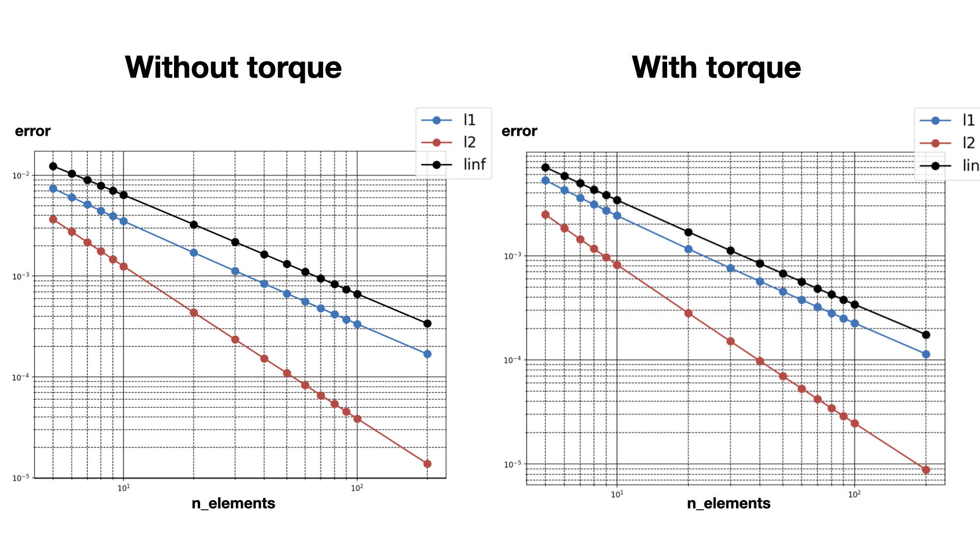
Modified Implementation

class EndpointForcesWithTorques(NoForces):
    """
    This class applies constant forces on the endpoint nodes.
    """

    def __init__(self, end_force, ramp_up_time=0.0):
        """

        Parameters
        ----------
        start_force: numpy.ndarray
            2D (dim, 1) array containing data with 'float' type.
            Force applied to first node of the rod-like object.
        end_force: numpy.ndarray
            2D (dim, 1) array containing data with 'float' type.
            Force applied to last node of the rod-like object.
        ramp_up_time: float
            Applied forces are ramped up until ramp up time.

        """
        self.end_force = end_force
        assert ramp_up_time >= 0.0
        self.ramp_up_time = ramp_up_time

    def apply_forces(self, system, time=0.0):
        factor = min(1.0, time / self.ramp_up_time)
        self.external_forces[..., -1] += self.end_force * factor

    def apply_torques(self, system, time: np.float64 = 0.0):
        factor = min(1.0, time / self.ramp_up_time)
        arm_length = system.lengths[...,-1]
        director = system.director_collection[..., -1]
        self.external_torques[..., -1] += np.cross(
            [0.0, 0.0, 0.5 * arm_length], director @ self.end_force
        )

Code Design: Mixin and Composition

Elastica package follows Mixin and composition design patterns that may be unfamiliar to users. Here is a collection of references that introduce the package design.

References

• stackoverflow discussion on Mixin

• example of Mixin: python collections

Hackathon Readme

NCSA-NVIDIA AI Hackathon held at the University of Illinois from March 7-8 2020.

Problem Statement

The objective is to train a model to move a (cyber)-octopus with two soft arms and a head to reach a target location, and then grab an object. The octopus is modeled as an assembly of Cosserat rods and is activated by muscles surrounding its arms. Input to the mechanical model is the activation signals to the surrounding muscles, which causes it to contract, thus moving the arms. The output of the model comes from the octopus’ environment. The mechanical model will be provided both for the octopus and its interaction with its environment. The goal is to find the correct muscle activation signals that make the octopus crawl to reach the target location and then make one arm to grab the object.

Progression of specific goals

These goals build on each other, you need to successfully accomplish all prior goals to get credit for later goals.

1. Make octopus crawl towards some direction. (5 points)

2. Make your octopus crawl to the target location. (7.5 points)

3. Make octopus to move the object using its arms. (7.5 points)

4. Have your octopus grab the object by wrapping one arm around the object. (10 points)

5. Make your octopus return to its starting location with the object. (20 points)

6. Generalize your policy to perform these tasks for an arbitrarily located object. (50 points)

Problem Context

Octopuses have flexible limbs made up of muscles with no internal bone structure. These limbs, know as muscular hydrostats, have an almost infinite number of degrees of freedom, allowing an octopus to perform complex actions with its arms, but also making them difficult to mathematically model. Attempts to model octopus arms are motivated not only by a desire to understand them biologically, but also to adapt their control ability and decision making processes to the rapidly developing field of soft robotics. We have developed a simulation package Elastica that models flexible 1-d rods, which can be used to represent octopus arms as a long, slender rod. We now want to learn methods for controlling these arms.

You are being provided with a model of an octopus that consists of two arms connected by a head. Each arm can be controlled independently. These arms are actuated through the contraction of muscles in the arms. This muscle activation produces a torque profile along the arm, resulting in movement of the arm. The arms interact with the ground through friction. Your goal is to teach the octopus to crawl towards an object, grab it, and bring it back to where the octopus started.

Controlling octopus arms with hierarchical basis functions

For this problem, we abstract the activation of the octopus muscles to the generation of a torque profile defined by the activation of a set of hierarchical radial basis function. Here we are using Gaussian basis functions.

There are three levels of these basis functions, with 1 basis function in the first level, 2 in the second level and 4 in the third, leading to 7 basis functions in set. These levels have different maximum levels of activation. The lower levels have larger magnitudes than the higher levels, meaning they represent bulk motion of the rod while the higher levels allow finer control of the rod along the interval. In the code, the magnitude of each level will be fixed but you can choose the amount of activation at each level by setting the activation level between -1 and 1.

There are two bending modes (in the normal and binormal directions) and a twisting mode (in the tangent direction), so we define torques in these three different directions and independently for each arm. This yields six different sets of basis functions that can be activated for a total of 42 inputs.

Overview of provided Elastica code

We are providing you the Elastica software package which is written in Python. Elastica simulates the dynamics and kinematics of 1-d slender rods. We have set up the model for you such that you do not need to worry about the details of the model, only the activation patterns of the muscle. In the provided examples/ArmWithBasisFunctions/two_arm_octopus_ai_imp.py file you will import the Environment class which will define and setup the simulation.

Environment has three relevant functions:

• Environment.reset(self): setups and initializes the simulation environment. Call this prior to running any simulations.

• Environment.step(self, activation_array_list, time): takes one timestep for muscle activations defined in activation_array_list.

• Environment.post_processing(self, filename_video): Makes 3D video based on saved data from simulation. Requires ffmpeg.
  We do not suggest changing Environment as it may cause unintended consequences to the simulation.

You will want to work within main() to interface with the simulations and develop your learning model. In main(), the first thing you need to define is the length of your simulation and initialize the environment. final_time is the length of time that your simulation will run unless exited early. You want to give your octopus enough time to complete the task, but too much time will lead to excessively long simulation times.

    # Set simulation final time
    final_time = 10.0

    # Initialize the environment
    target_position = np.array([-0.4, 0.0, 0.5])
    env = Environment(final_time, target_position, COLLECT_DATA_FOR_POSTPROCESSING=True)
    total_steps, systems = env.reset()

With your system initialized, you are now ready to perform the simulation. To perform the simulation there are two steps:

1. Evaluate the reward function and define the basis function activations

2. Perform time step

There is also a user defined stopping condition. When met, this will immediately end the simulation. This can be useful to end the simulation if the octopus successfully complete the task early, or has a sufficiently low reward function that there is no point continuing the simulation.

    for i_sim in tqdm(range(total_steps)):
	""" Learning loop """
	if i_sim % 200:
           """ Add your learning algorithm here to define activation """
           # This will be based on your observations of the system and 
           # evaluation of your reward function.  
           shearable_rod = systems[0]
           rigid_body = systems[1]   
           reward = reward_function()   
           activation = segment_activation_function()

        """ Perform time step """
        time, systems, done = env.step(activation, time)

        """ User defined condition to exit simulation loop """
        done = user_defined_condition_function(reward, systems, time)
        if done:
            break

The state of the octopus is available in shearable_rod. The octopus consists of a series of 121 nodes. Nodes 0-49 relate to one arm, nodes 50-70 relate to the head, and nodes 71-120 relate to the second arm. shearable_rod.position_collection returns an array with entries relating to the position of each node. The state of the target object is available in rigid_body.

It is important to properly define the activation function. It consists of a list of lists defining the activation of the two arms in each of the the three modes of deformation. The activation function should be a list with three entries for the three modes of deformation. Each of these entries is in turn a list with two entries, which are arrays of the basis function activations for the two arms.

    activation = [
        [arm_1_normal,   arm_2_normal],    # activation in normal direction
        [arm_1_binormal, arm_2_binormal],  # activation in binormal direction
        [arm_1_tangent,  arm_2_tangent],   # activation in tangent direction
        ]

Each activation array has 7 entries that relate to the activation of different basis functions. The ordering goes from the top level to the bottom level of the hierarchy. Each entry can vary from -1 to 1.

activation_array[0]  – One top level muscle segment
activation_array[1:3] – Two mid level muscle segment
activation_array[3:7] – Four bottom level muscle segment

A few practical notes

1. To save a video of the octopus with Environment.post_processing(), you need to install ffmeg. You can download and install it here.

2. The timestep size is set to 40 μs. This is necessary to keep the simulation stable, however, you may not need to update your muscle activations that often. Varying the learning time step will change how often your octopus updates its behaviour.

3. There is a 15-20 second startup delay while the simulation is initialized. This is a one time cost whenever the Python script is run and resetting the simulation using .rest() does not incur this delay for subsequent simulations.

4. We suggest installing requirements.txt and optional-requirements.txt, to run Elastica without any problem.

---

Indices and tables

• Index

• Module Index

• Search Page